Exploring the possibilities of Gaussian splatting for navigation in large landscapes.
Capture and navigate a real landscape
In the vast array of technological tools that have flourished in recent years as a result of the accelerated development of deep learning, alongside LLMs and diffusion algorithms, other work is likely to transform their respective fields in the years to come.
These include neural radiance fields (or NeRFs), and the 3D gaussian splatting method. These two methods, and their many derivatives and improvements, can be seen as extensions to photogrammetry. The idea is to use an image sequence, taken from photos or videos, to generate a three-dimensional representation of the captured scene. Like the deep learning applications mentioned above, these two methods rely on a process of training and optimization/error minimization. Note, however, that while NeRFs are indeed a deep learning application, 3D gaussian splatting is not.
While the result of implementing photogrammetry is usually a point cloud or, ideally, a textured mesh (as proposed by software such as Meshroom and RealityCapture), NeRFs or 3D gaussian splatting (which I’ll shorten to gsplat from here on in) methods offer significantly different representations. Without going into too much detail, NeRFs use a neural network to represent the way light propagates in a 3D volume. These methods therefore have no notion of geometry, but are capable of generating plausible new points of view. As for gsplats, these methods can be likened to point cloud representations, but this time using 3D Gaussians whose color and shape characteristics (again simplifying) enable a more accurate representation of the captured scene than these. More details on the workings of gsplats can be found on the Hugging Face blog.
As part of an upcoming project, we plan to enable visitors to an immersive space to navigate freely in a real landscape. Due to the complexity of the potential geometry and the dimensions of the landscape, traditional photogrammetry is not an option. This is therefore an opportunity to evaluate the potential of gsplat to create a live navigable representation, based on drone shots. NeRFs are not suitable for this purpose, due to the computational resources required to obtain a sufficient refresh rate, a problem that gsplat does not present.
Implementing tests
To evaluate this representation, we need :
- a suite of tools for generating and visualizing 3D Gaussians
- a sequence of landscape images
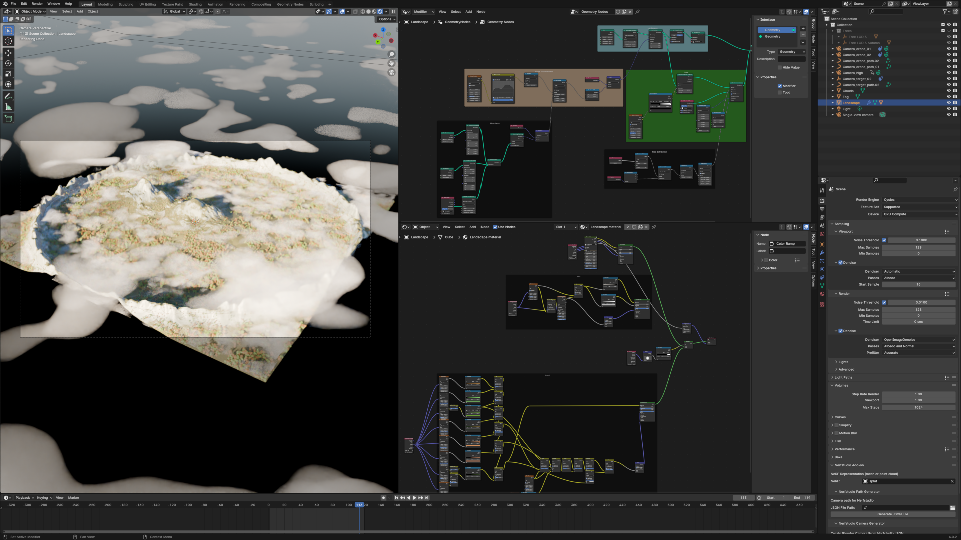
For the second point, as I didn’t have a drone or a mountainous landscape at my disposal, I opted for a simulation from scratch. It’s beyond the scope of this article, but I used Blender to generate a 1km² mountain landscape. There are many tutorials on the subject, the most recent taking advantage of geometry nodes for rather satisfactory results. For the curious, the Blender scene is available here. The image at the beginning of this article shows the scene loaded into Blender.
As for the first point, after having reviewed the state of the art of the available tools, I stopped at nerfstudio. As its name does not suggest, nerfstudio implements several scene representation methods, including 3D gaussian splatting. And unlike INRIA’s initial implementation, which has a free license for non-commercial use, nerfstudio’s is licensed under Apache, which allows all types of use. Another advantage is that the project is supported by a very active community, which augurs well for long-term support.
The actual installation of nerfstudio is beyond the scope of this article, especially as it is likely to change over time. The documentation is comprehensive enough for anyone familiar with the terminal and the Python ecosystem to find their way around. However, here’s a look at what needs to be installed, on a machine with an NVIDIA GPU running Linux (unfortunately nerfstudio can’t work with AMD GPUs):
  # Installation of Miniconda
  mkdir -p ~/miniconda3
  wget https://repo.anaconda.com/miniconda/Miniconda3-latest-Linux-x86_64.sh -O ~/miniconda3/miniconda.sh
  # Tip: answer 'no' to Conda's default activation
  # to maintain control over your environment
  bash ~/miniconda3/miniconda.sh -b -u -p ~/miniconda3
  rm -rf ~/miniconda3/miniconda.sh

  # Activation of Conda, considering Bash is used as the shell
  eval "$(${HOME}/Apps/miniconda3/bin/conda shell.bash hook)"

  # Installation of nerfstudio and its dependencies
  conda create --name nerfstudio -y python=3.8
  conda activate nerfstudio
  python3 -m pip install --upgrade pip

  pip uninstall torch torchvision functorch tinycudann
  pip install torch==2.1.2+cu118 torchvision==0.16.2+cu118 --extra-index-url https://download.pytorch.org/whl/cu118
  conda install -c "nvidia/label/cuda-11.8.0" cuda-toolkit
  pip install ninja git+https://github.com/NVlabs/tiny-cuda-nn/#subdirectory=bindings/torch
  pip install nerfstudio

  # Installation of COLMAP, used to align images
  conda install colmap
  # On some computers, COLMAP needs CUDA 12.0, so if that's your case:
  conda install -c "nvidia/label/cuda-12.0.0" cuda-toolkit
Once installed, the procedure for generating a representation from a sequence of images is as follows:
  # Activation of Conda environment
  conda activate nerfstudio

  # Image alignment and training
  ns-process-data images --data /path/to/image/sequence --output-dir ./work-dir

  # Training
  ns-train splatfacto --data work-dir
The training result will be stored in ./outputs/work-dir/splatfacto/${RUN DATE}, and it is possible to view the live representation by opening your preferred browser at https://localhost:7007.
Tests and results
Several camera paths were tested, simulating the path a drone might take across a real landscape. For each path, several hundred images were rendered, at varying frequencies and resolutions, depending on each test. The following parameters were evaluated:
- type of path, including camera orientation,
- frequency of shots,
- resolution of shots,
- number of shots,
- the number of iterations in the optimization process,
- and the number of Gaussians generated.
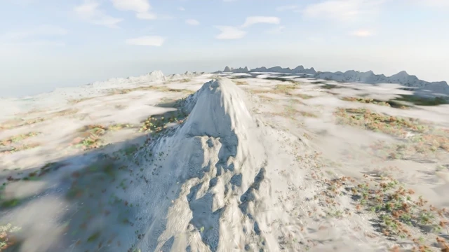
Overall, the results are quite impressive. The representation is very interesting and the rendering is very good, though easily distinguishable from the original images. There’s still some way to go to achieve a result that’s hard to distinguish from the original images, whether in terms of the optimization algorithms or, just as likely, my own mastery of the training process. Here’s an animation of one of the resulting representations, which is fluidly manipulated on my aging laptop with an integrated Intel GPU:
There are a few points to bear in mind for future tests. Firstly, representation accuracy is not linearly related to image resolution. This is no surprise, as it is also the case with traditional photogrammetry methods. The nerfstudio documentation suggests limiting the image size to 1600 pixels (and by default forces a resizing of the image if this is not possible). In my tests with 3200x2400 images, the representation was not much more defined than at 1600x1200.
The overlap ratio between successive images is an important parameter. The rule of thumb that says you should aim for 1/3 overlap between two successive images is still valid, and if the scene features many small objects, you shouldn’t hesitate to go beyond this to ensure they are better represented. It is also important to have diversity in viewpoints, and in particular to take advantage of changes in parallax. In concrete terms, this translates into the importance of favoring orthogonal displacements in relation to the objects you wish to capture: results will be less good (or even impossible to train) if the camera is pointing in the direction of displacement, in particular.
In direct relation to the overlap rate, we recommend a camera with the widest possible field of view. It’s even possible to train with panoramic images (equirectangular projection). I haven’t tested it yet, but the prospects are interesting. See the nerfstudio documentation on this subject.
Also, while there may be a tendency to multiply images to promote large overlays, it’s important to bear in mind that these methods are very memory-hungry. I had to reserve 48GB of system memory for a training session with 780 images at 3200x1600.
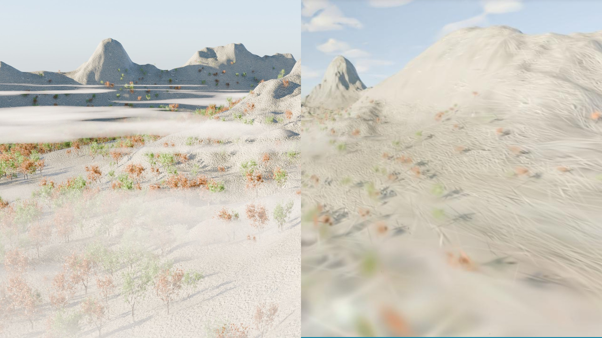
To give some perspective on gsplat’s capabilities, if the previous animation is difficult to distinguish from the original scene, it is more obvious in the following two renders to determine which has been made from the original Blender scene, and which from the 3D Gaussian representation. This is obviously linked to the viewpoints of the images used for training, but it’s easy to see that the intended use will have a major impact on the shots.
And finally, having manipulated the parameters under many different conditions, it’s obvious that the default settings are a very good starting point. So it’s best to work with them and improve your image sequence until you’re satisfied, before diving into time-consuming experiments that can be difficult to compare.
Improving the results
Speaking of comparisons, I strongly recommend the use of TensorBoard, one of nerfstudio’s training visualization modes. Using it requires a little digging in the documentation, but here’s the gist:
  # Installation of TensorBoard
  pip3 install tensorboard

  # Training must be started with another viewer
  ns-train splatfacto --vis viewer+tensorboard --data work-dir

  # During or after training, launch TensorBoard
  cd outputs/work-dir/splatfacto/${RUN DATE}/
  tensorboard --logdir=outputs/work-dir/splatfacto/${RUN DATE}/
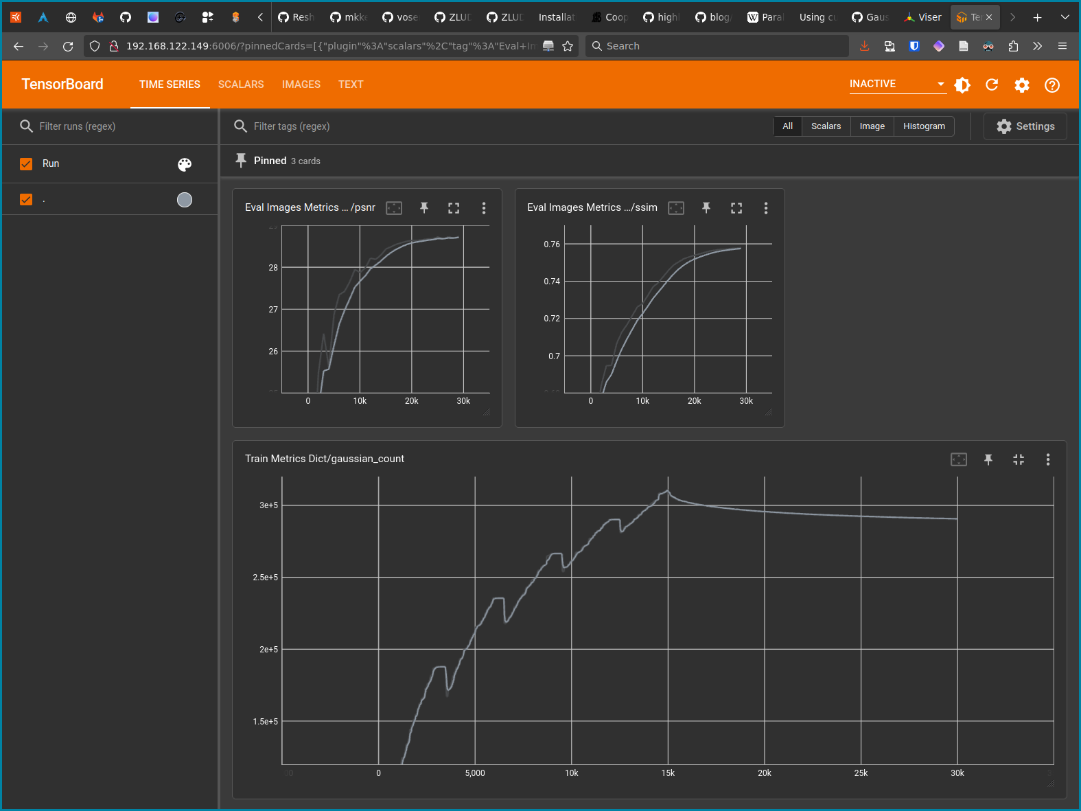
The TensorBoard interface can then be accessed from https://localhost:6006. In my experience, the main metrics to track are SSIM and PSNR in the Eval Images Metrics Dicts section, and gaussian_count in the Train Metrics Dict section. The first two measure similarity and signal-to-noise ratio, and are an indication of representation quality. The third simply indicates the number of Gaussians in the representation, which will have a direct impact on its size and visualization performance. In the following image, we can see that SSIM and PSNR increase progressively until they reach a plateau:
Closing notes
After these few tests, I’m still convinced that gsplats will have many applications and a major influence on the world of graphics computing and virtual reality in the years to come. Just as much as NeRFs, in fact, even if for the time being they are difficult to manipulate in real time.
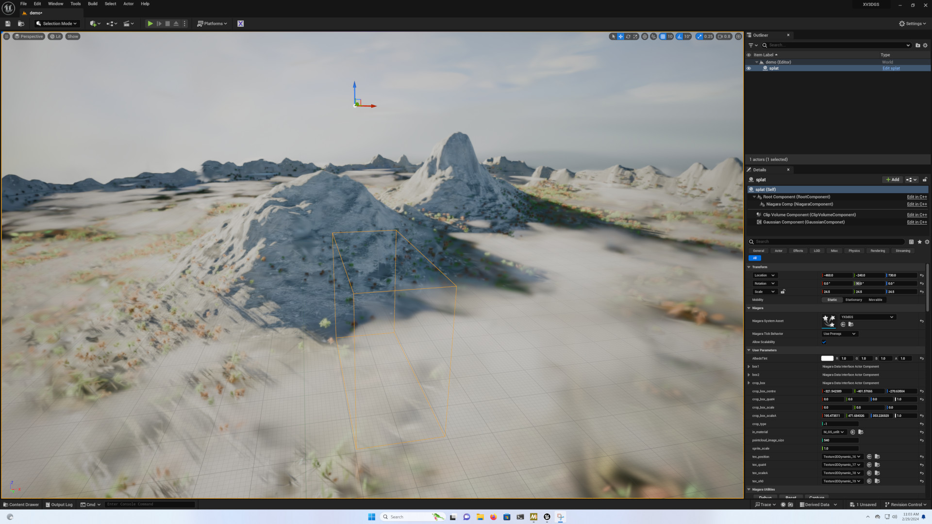
There are many points I haven’t covered in this article, and in particular everything to do with use in other software. There are addons for several, the most advanced currently being for Unreal Engine, including XV3DGS-UEPlugin, 3D gaussian splatting rendering for UE and the Luma-AI addon.
The situation is less rosy for other tools, although it will certainly improve. One example is the Gaussian splatting Blender addon. For more sources on the subject, I recommend the comprehensive repository Awesome 3D gaussian splatting.